Exploratory Data Analysis

This report documents the exploratory analysis that motivated the feature engineering decisions in the EDA recipe. Each section examines the relationship between a predictor and log sale price, identifies nonlinearities or skew, and explains the transformation chosen to address it. The goal was to make informed, interpretable decisions rather than relying on automated transformation strategies alone.

Outcome Variable

Code

p1 <- ggplot(miami, aes(x = exp(sale_prc_log))) +
  geom_histogram(bins = 60, fill = "steelblue", color = "white") +
  scale_x_continuous(labels = scales::dollar_format()) +
  labs(title = "Original scale", x = "Sale price", y = "Count")

p2 <- ggplot(miami, aes(x = sale_prc_log)) +
  geom_histogram(bins = 60, fill = "steelblue", color = "white") +
  labs(title = "Log scale", x = "log(Sale price)", y = "Count")

p1 + p2 +
  plot_annotation(title = "Sale price distribution before and after log transformation")

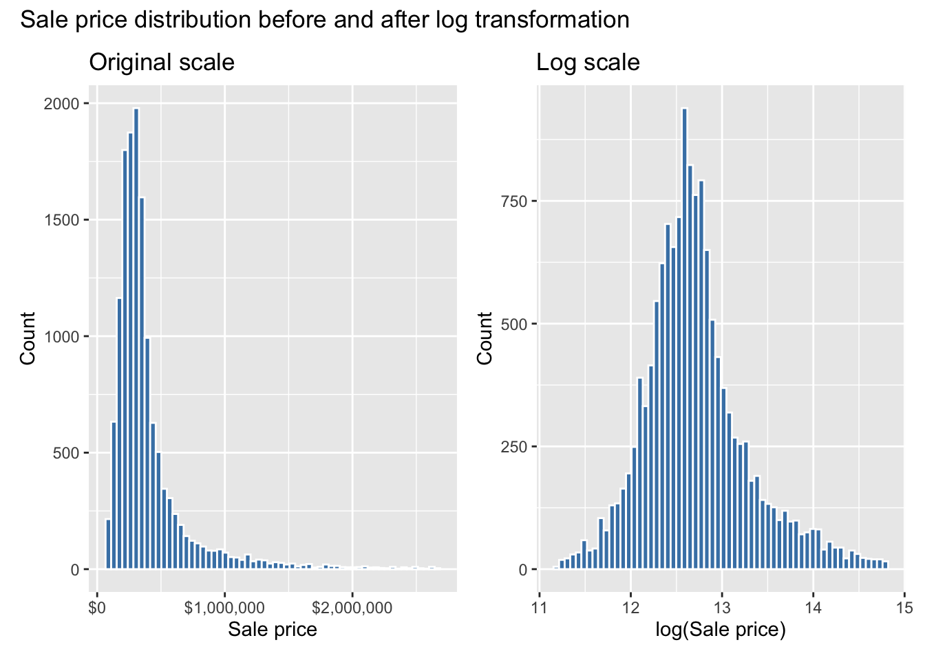
Sale price on the original scale is strongly right-skewed, with the bulk of properties clustered below $500,000 and a long tail extending toward $2.5 million. The log transformation produces a near-symmetric, approximately normal distribution. All modeling is performed on log sale price and predictions are back-transformed with exp() when dollar-scale interpretation is needed.

Location Effects

Code

p1 <- ggplot(miami, aes(x = latitude, y = sale_prc_log)) +
  geom_point(alpha = 0.1, size = 0.5) +
  geom_smooth(color = "red") +
  labs(title = "Latitude vs log price", x = "Latitude", y = "log(Sale price)")

p2 <- ggplot(miami, aes(x = longitude, y = sale_prc_log)) +
  geom_point(alpha = 0.1, size = 0.5) +
  geom_smooth(color = "red") +
  labs(title = "Longitude vs log price", x = "Longitude", y = "log(Sale price)")

p1 + p2

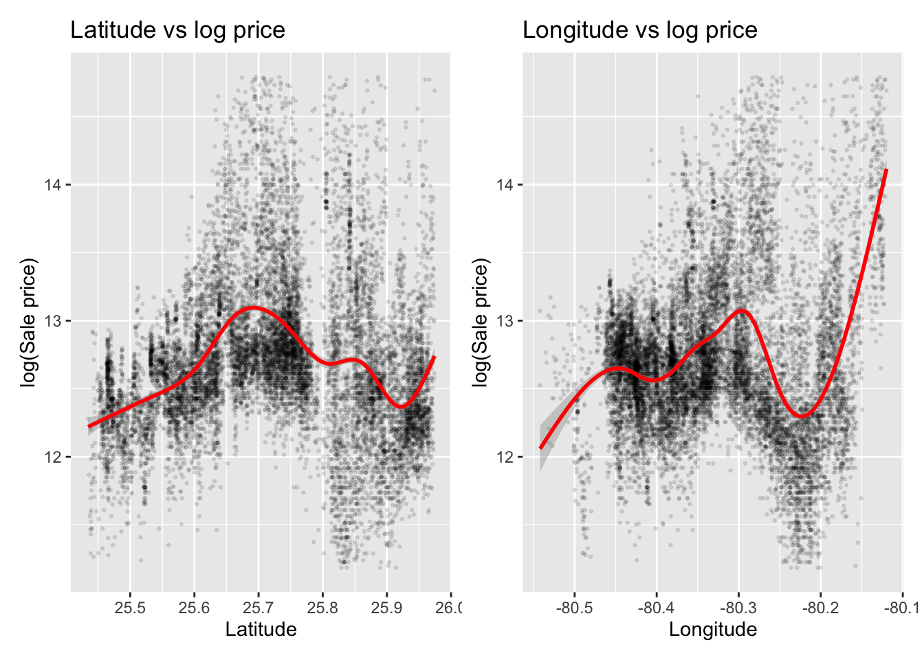
The latitude relationship is clearly nonlinear. Prices peak in the middle latitudes and drop off at both ends, reflecting the concentration of higher-value neighborhoods in central Miami. A single linear term cannot capture this curve, motivating the use of a natural spline with 4 degrees of freedom in the EDA recipe.

The longitude relationship shows a U-shape, with lower prices in the middle longitudes and higher prices toward both extremes. This pattern likely reflects the premium commanded by properties near the coast on either side of the peninsula. Squaring longitude captures this U-shape with a single additional term, which is a more parsimonious solution than a spline for a clean quadratic relationship.

Distance Variables

Code

p1 <- ggplot(miami, aes(x = ocean_dist, y = sale_prc_log)) +
  geom_point(alpha = 0.1, size = 0.5) +
  geom_smooth(color = "red") +
  labs(title = "Ocean distance", x = "Distance (ft)", y = "log(Sale price)")

p2 <- ggplot(miami, aes(x = log(ocean_dist), y = sale_prc_log)) +
  geom_point(alpha = 0.1, size = 0.5) +
  geom_smooth(color = "red") +
  labs(title = "log(Ocean distance)", x = "log(Distance)", y = "log(Sale price)")

p3 <- ggplot(miami, aes(x = hwy_dist, y = sale_prc_log)) +
  geom_point(alpha = 0.1, size = 0.5) +
  geom_smooth(color = "red") +
  labs(title = "Highway distance", x = "Distance (ft)", y = "log(Sale price)")

p4 <- ggplot(miami, aes(x = log(hwy_dist + 1), y = sale_prc_log)) +
  geom_point(alpha = 0.1, size = 0.5) +
  geom_smooth(color = "red") +
  labs(title = "log(Highway distance)", x = "log(Distance)", y = "log(Sale price)")

(p1 + p2) / (p3 + p4)

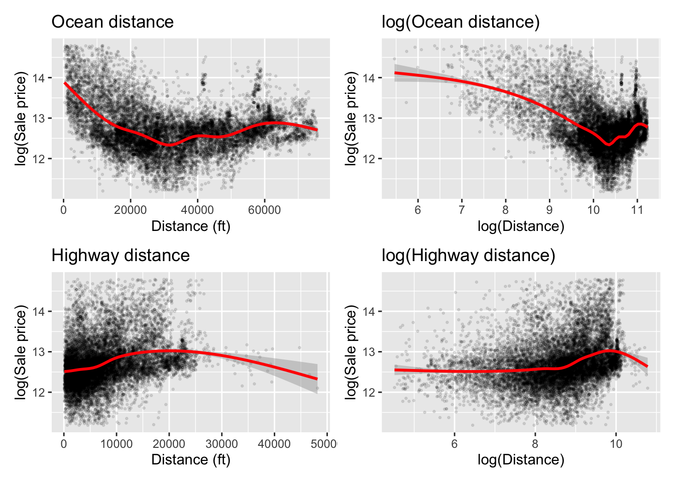
Highway distance shows strong right skew on the original scale, with a steeply diminishing relationship that flattens quickly. Log-transforming highway distance straightens this relationship considerably, producing a much more linear pattern. This is the cleanest transformation in the EDA recipe and produces the most consistent improvement across model families.

Ocean distance presents a more complex pattern. Even after log-transforming, the smoothed curve retains meaningful curvature that a linear term cannot adequately capture. This motivates the use of a natural spline with 4 degrees of freedom, which gives the model enough flexibility to follow the nonlinear price gradient as distance from the ocean increases.

Special Features Value

Code

p1 <- ggplot(miami, aes(x = spec_feat_val, y = sale_prc_log)) +
  geom_point(alpha = 0.1, size = 0.5) +
  geom_smooth(color = "red") +
  labs(title = "Special features value", x = "Value ($)", y = "log(Sale price)")

p2 <- ggplot(miami, aes(x = sqrt(spec_feat_val), y = sale_prc_log)) +
  geom_point(alpha = 0.1, size = 0.5) +
  geom_smooth(color = "red") +
  labs(title = "sqrt(Special features value)", x = "sqrt(Value)", y = "log(Sale price)")

p1 + p2

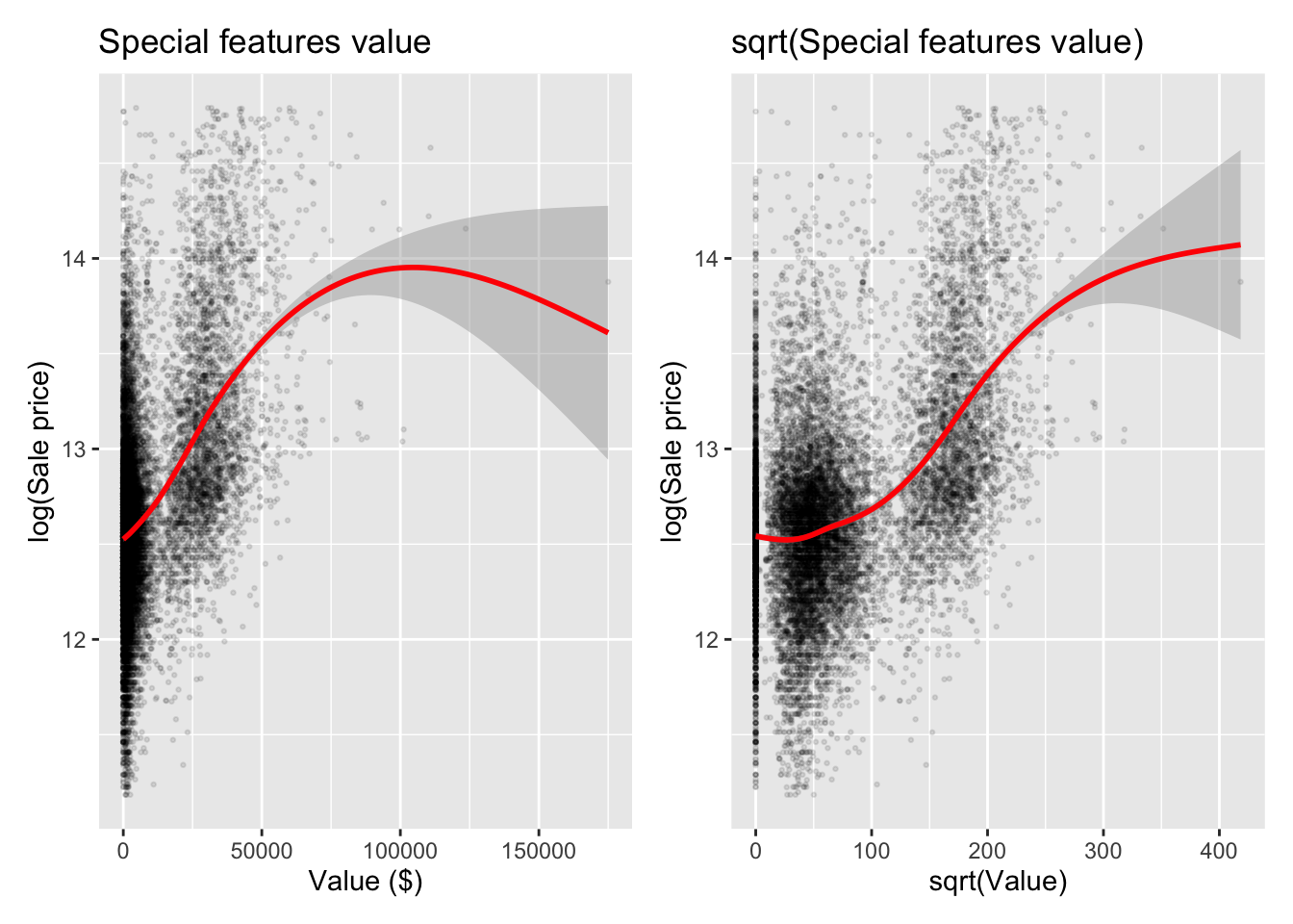
Special features value is heavily concentrated at zero, with a long right tail for properties that have pools, docks, or other premium amenities. On the original scale the relationship with log price is steep and nonlinear. The square root transformation compresses the tail, reduces skew, and produces a noticeably more linear relationship. A log transformation was considered but performs worse here because of the large number of zero values, which would require an offset and add complexity without improving the fit.

Structural Variables

Code

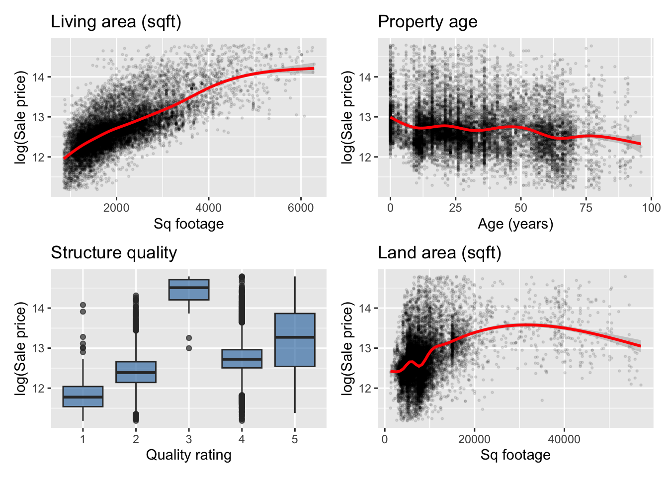
p1 <- ggplot(miami, aes(x = tot_lvg_area, y = sale_prc_log)) +
  geom_point(alpha = 0.1, size = 0.5) +
  geom_smooth(color = "red") +
  labs(title = "Living area (sqft)", x = "Sq footage", y = "log(Sale price)")

p2 <- ggplot(miami, aes(x = age, y = sale_prc_log)) +
  geom_point(alpha = 0.1, size = 0.5) +
  geom_smooth(color = "red") +
  labs(title = "Property age", x = "Age (years)", y = "log(Sale price)")

p3 <- ggplot(miami, aes(x = structure_quality, y = sale_prc_log)) +
  geom_boxplot(fill = "steelblue", alpha = 0.7) +
  labs(title = "Structure quality", x = "Quality rating", y = "log(Sale price)")

p4 <- ggplot(miami, aes(x = lnd_sqfoot, y = sale_prc_log)) +
  geom_point(alpha = 0.1, size = 0.5) +
  geom_smooth(color = "red") +
  labs(title = "Land area (sqft)", x = "Sq footage", y = "log(Sale price)")

(p1 + p2) / (p3 + p4)

Living area has a strong positive relationship with log price, as expected. The relationship is approximately linear on the log scale and does not require additional transformation. Property age shows a nonlinear pattern. Very new and very old properties both command premiums relative to mid-age properties. New construction is valued for modern amenities, while older properties in Miami often reflect historic or architecturally desirable stock. Structure quality shows a clear ordinal gradient with limited overlap between adjacent levels, confirming it is one of the strongest property-level predictors. Land area has a weaker and noisier relationship with price than living area, suggesting that buyers in this market value interior space more than lot size.

Correlation Overview

Code

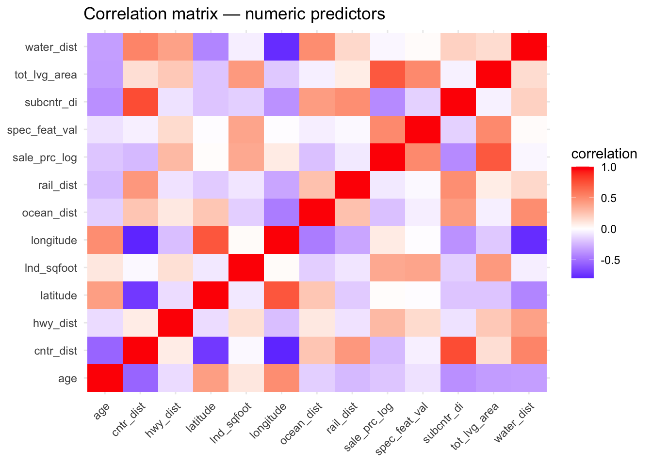
miami %>%
  select(where(is.numeric)) %>%
  cor() %>%
  as.data.frame() %>%
  rownames_to_column("var1") %>%
  pivot_longer(-var1, names_to = "var2", values_to = "correlation") %>%
  ggplot(aes(x = var1, y = var2, fill = correlation)) +
  geom_tile() +
  scale_fill_gradient2(low = "blue", mid = "white", high = "red", midpoint = 0) +
  theme_minimal() +
  theme(axis.text.x = element_text(angle = 45, hjust = 1)) +
  labs(title = "Correlation matrix — numeric predictors", x = NULL, y = NULL)

Ocean distance and water distance are highly correlated, as expected given Miami’s coastal geography. Latitude and longitude show moderate correlation with several distance variables, reflecting the city’s linear layout along the coast. The distance variables as a group show meaningful multicollinearity, which is expected and handled naturally by tree-based models. For linear models, this multicollinearity contributes to the weaker performance seen in the cross-validation results, as correlated predictors inflate coefficient variance and reduce interpretability. The interactions recipe addresses this by compressing the predictor space with PCA, though the EDA recipe ultimately proves more effective by addressing the nonlinearity directly.