Model Results & Final Evaluation

Cross-Validation Summary

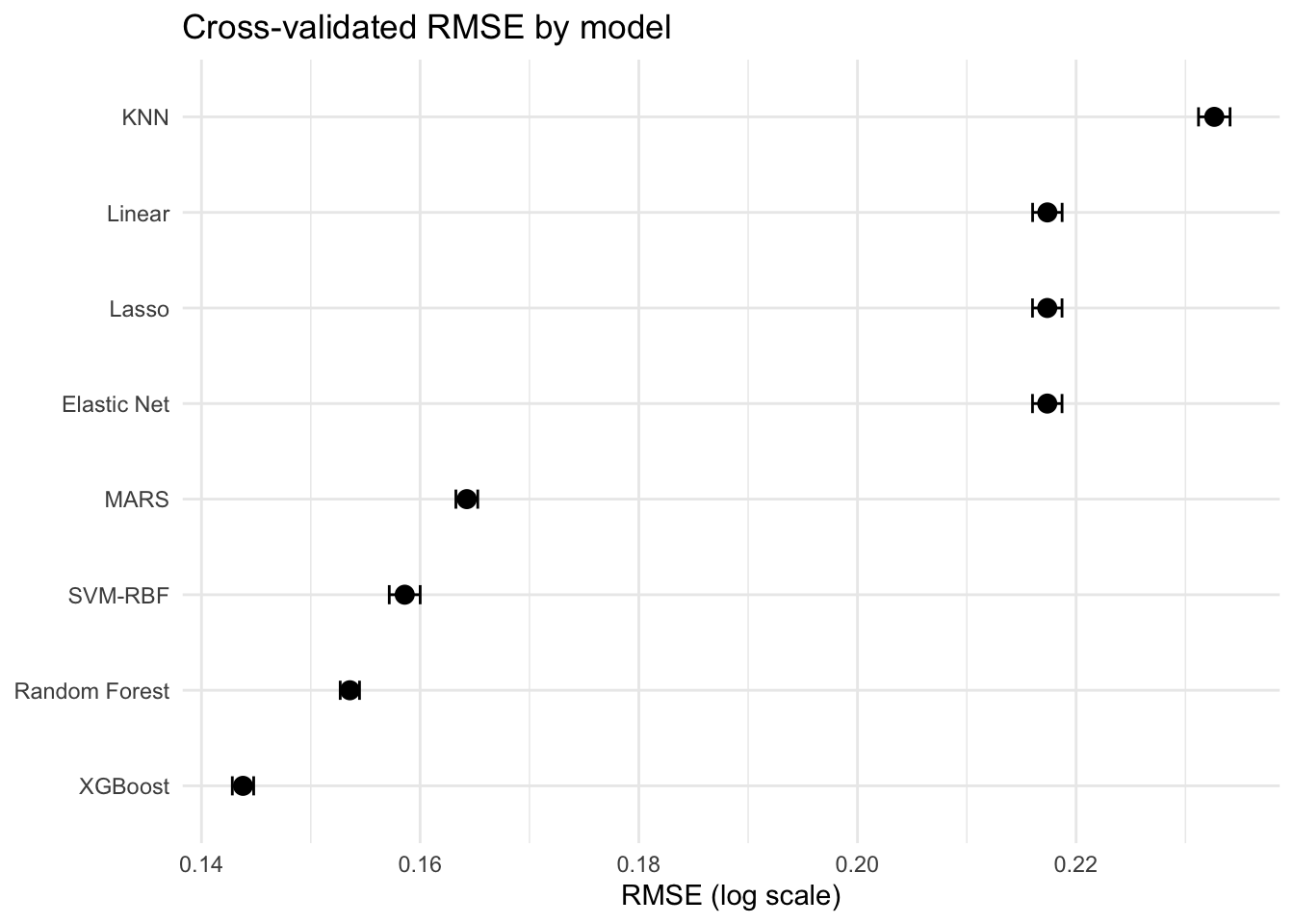
Eight model families were evaluated using 5-fold cross-validation with 3 repeats, stratified on log sale price. Each model was paired with the preprocessing recipe that produced its best performance. RMSE on the log scale is the primary comparison metric throughout.

Code

# Load best result from each model
results <- tribble(
  ~model,          ~recipe,        ~file,
  "XGBoost",       "EDA",          "results/tuning/xgb_eda.rds",
  "Random Forest", "EDA",          "results/tuning/rf_eda.rds",
  "SVM-RBF",       "EDA",          "results/tuning/svm_eda.rds",
  "MARS",          "EDA",          "results/tuning/mars_eda.rds",
  "Linear",        "Interactions", "results/tuning/lm_interactions.rds",
  "Elastic Net",   "Interactions", "results/tuning/en_interactions.rds",
  "Lasso",         "Interactions", "results/tuning/lasso_interactions.rds",
  "KNN",           "EDA",          "results/tuning/knn_eda.rds"
)

extract_best_rmse <- function(file) {
  result <- read_rds(file)
  best   <- show_best(result, metric = "rmse", n = 1)
  tibble(mean = best$mean, std_err = best$std_err)
}

cv_summary <- results %>%
  mutate(metrics = map(file, extract_best_rmse)) %>%
  unnest(metrics) %>%
  select(model, recipe, mean, std_err) %>%
  arrange(mean)

cv_summary %>%
  gt() %>%
  cols_label(
    model   = "Model",
    recipe  = "Recipe",
    mean    = "CV RMSE",
    std_err = "Std Error"
  ) %>%
  fmt_number(columns = c(mean, std_err), decimals = 4) %>%
  tab_style(
    style = cell_fill(color = "#e8f5e9"),
    locations = cells_body(rows = 1)
  ) %>%
  tab_header(title = "Cross-Validation RMSE by Model")

Cross-Validation RMSE by Model
Model	Recipe	CV RMSE	Std Error
XGBoost	EDA	0.1438	0.0010
Random Forest	EDA	0.1536	0.0009
SVM-RBF	EDA	0.1586	0.0014
MARS	EDA	0.1643	0.0010
Elastic Net	Interactions	0.2174	0.0014
Lasso	Interactions	0.2174	0.0014
Linear	Interactions	0.2174	0.0014
KNN	EDA	0.2326	0.0014

Code

cv_summary %>%
  mutate(model = fct_reorder(model, mean)) %>%
  ggplot(aes(x = mean, y = model)) +
  geom_point(size = 3) +
  geom_errorbarh(
    aes(xmin = mean - std_err, xmax = mean + std_err),
    height = 0.2
  ) +
  labs(
    title = "Cross-validated RMSE by model",
    x     = "RMSE (log scale)",
    y     = NULL
  ) +
  theme_minimal()

Tree-based models substantially outperform linear and distance-based approaches. The performance gap between XGBoost (0.144) and the best linear model (0.217) is large enough to confirm that the data contains nonlinear structure that coefficients cannot capture. KNN underperforms despite being nonparametric, likely because the distance calculations are sensitive to the high-dimensional, correlated predictor space. The EDA recipe wins or ties for first across every flexible model family. This is the most important finding in this comparison, as it validates the value of domain-informed feature engineering over automated alternatives.

Winning Model: XGBoost + EDA Recipe

Code

xgb_eda_result <- read_rds("results/tuning/xgb_eda.rds")

best_params <- select_best(xgb_eda_result, metric = "rmse")

final_spec <- boost_tree(
  trees          = best_params$trees,
  tree_depth     = best_params$tree_depth,
  learn_rate     = best_params$learn_rate,
  loss_reduction = best_params$loss_reduction,
  min_n          = best_params$min_n
) %>%
  set_engine("xgboost") %>%
  set_mode("regression")

final_workflow <- workflow() %>%
  add_recipe(recipe_eda) %>%
  add_model(final_spec)

# Fit on full training set
final_fit <- fit(final_workflow, data = miami_train)

write_rds(final_fit, "results/final_fit.rds")
message("✓ Final model fit saved.")

The best hyperparameters were selected by minimizing cross-validated RMSE. The final model is trained on the full training set using these parameters before evaluation on the held-out test set. The test set is touched exactly once.

Test Set Evaluation

Code

test_preds <- predict(final_fit, new_data = miami_test) %>%
  bind_cols(miami_test) %>%
  mutate(
    sale_prc_actual    = exp(sale_prc_log),
    sale_prc_predicted = exp(.pred)
  )

# Metrics on log scale
log_metrics <- test_preds %>%
  metrics(truth = sale_prc_log, estimate = .pred) %>%
  filter(.metric %in% c("rmse", "rsq", "mae"))

# Metrics on dollar scale
dollar_metrics <- test_preds %>%
  metrics(truth = sale_prc_actual, estimate = sale_prc_predicted) %>%
  filter(.metric %in% c("rmse", "mae"))

log_metrics %>%
  bind_rows(dollar_metrics) %>%
  gt() %>%
  cols_label(.metric = "Metric", .estimator = "Type", .estimate = "Value") %>%
  fmt_number(columns = .estimate, decimals = 4) %>%
  tab_header(title = "Test Set Performance — XGBoost + EDA Recipe")

Test Set Performance — XGBoost + EDA Recipe
Metric	Type	Value
rmse	standard	0.1415
rsq	standard	0.9363
mae	standard	0.0973
rmse	standard	89,863.7891
mae	standard	42,294.4989

The test RMSE of 0.1415 is close to the cross-validated estimate of 0.1440, confirming that the model generalizes well and that the CV procedure was not optimistic. The model explains 93.6% of variance in log sale price. On the dollar scale, the median absolute error of $42,294 provides the most practically interpretable summary of prediction accuracy.

Predicted vs Actual

Code

ggplot(test_preds, aes(x = sale_prc_actual, y = sale_prc_predicted)) +
  geom_point(alpha = 0.3, size = 0.8) +
  geom_abline(color = "red", linetype = "dashed") +
  scale_x_continuous(labels = scales::dollar_format()) +
  scale_y_continuous(labels = scales::dollar_format()) +
  labs(
    title = "Predicted vs actual sale price",
    x     = "Actual price",
    y     = "Predicted price"
  ) +
  theme_minimal()

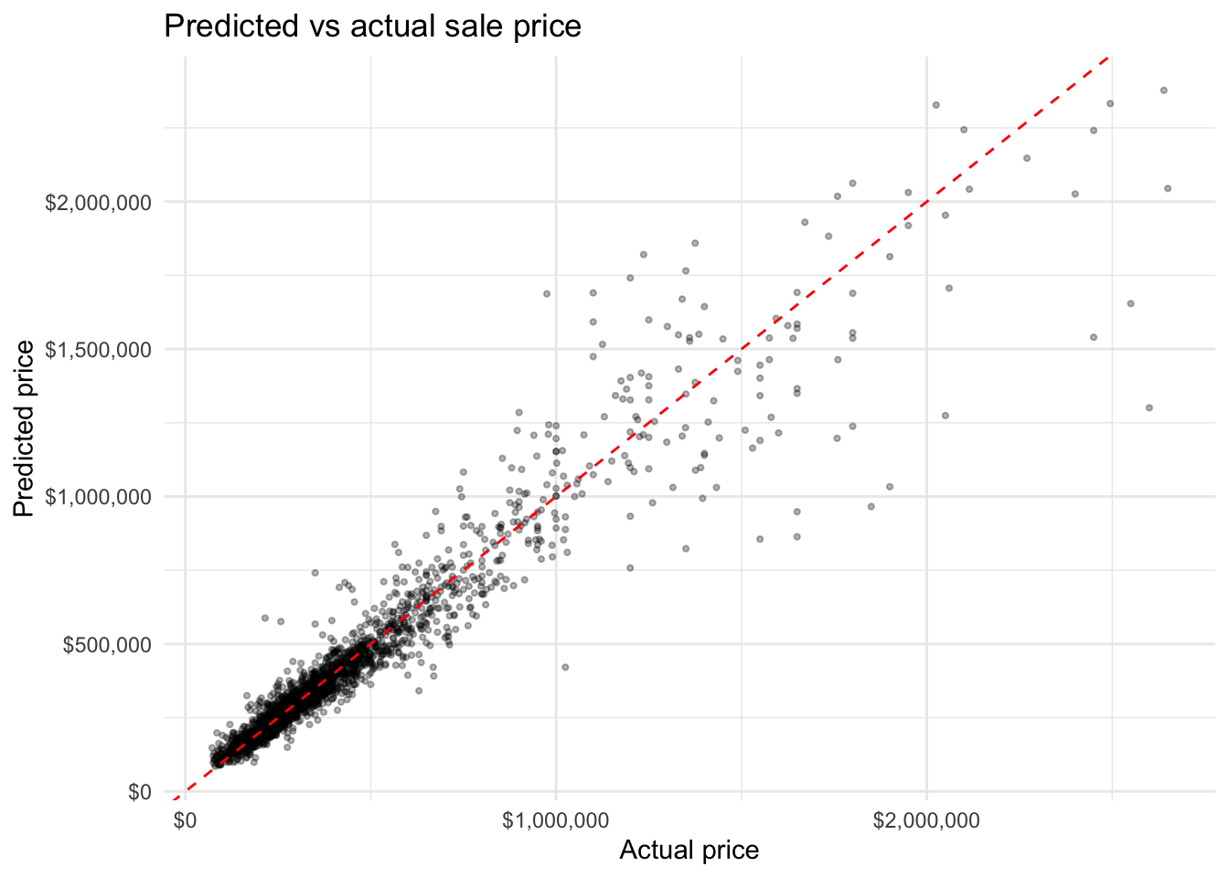
Predictions align closely with actual prices across most of the range. The model performs well for the majority of properties, which fall below $750,000. At the high end, a small number of luxury properties are underpredicted which is a common pattern when training data contains few examples of extreme values and the model has limited information to extrapolate beyond the bulk of the distribution.

Residual Analysis

Code

test_preds <- test_preds %>%
  mutate(residual = sale_prc_log - .pred)

p1 <- ggplot(test_preds, aes(x = .pred, y = residual)) +
  geom_point(alpha = 0.3, size = 0.8) +
  geom_hline(yintercept = 0, color = "red", linetype = "dashed") +
  labs(title = "Residuals vs fitted", x = "Fitted (log scale)", y = "Residual") +
  theme_minimal()

p2 <- ggplot(test_preds, aes(x = residual)) +
  geom_histogram(bins = 50, fill = "steelblue", color = "white") +
  labs(title = "Residual distribution", x = "Residual", y = "Count") +
  theme_minimal()

p1 + p2

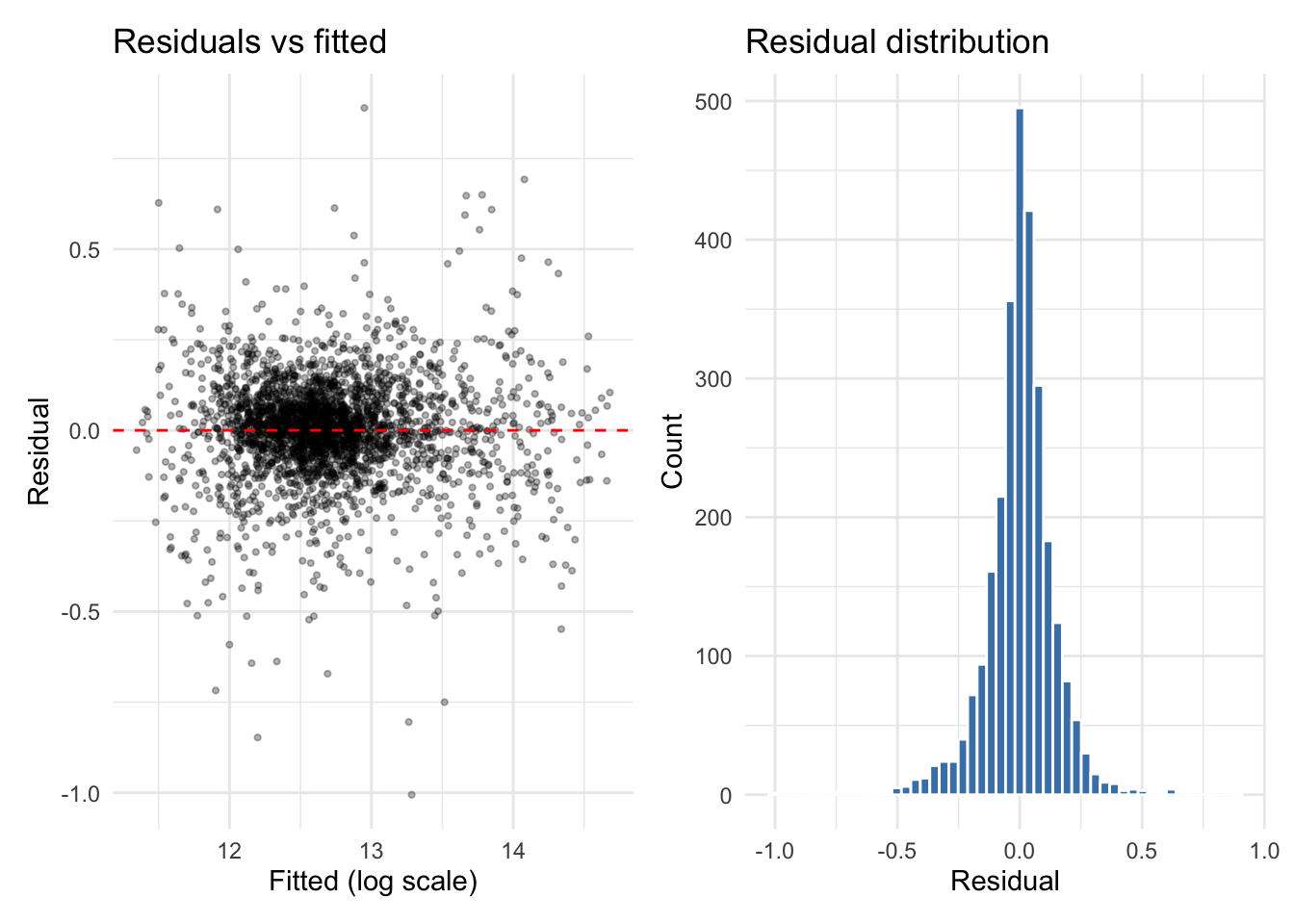
Residuals are approximately centered at zero with no strong systematic pattern against fitted values, indicating the model is not consistently over or underpredicting at any price level. The distribution is approximately normal with a slight right skew, driven by the same high-value outliers visible in the predicted vs actual plot. The absence of a funnel shape or nonlinear pattern in the residuals vs fitted plot confirms that the log transformation of the outcome was appropriate and that variance is reasonably stable across the prediction range.

Variable Importance

Code

final_fit %>%
  extract_fit_parsnip() %>%
  vip(num_features = 15) +
  labs(title = "Top 15 predictors — XGBoost feature importance") +
  theme_minimal()

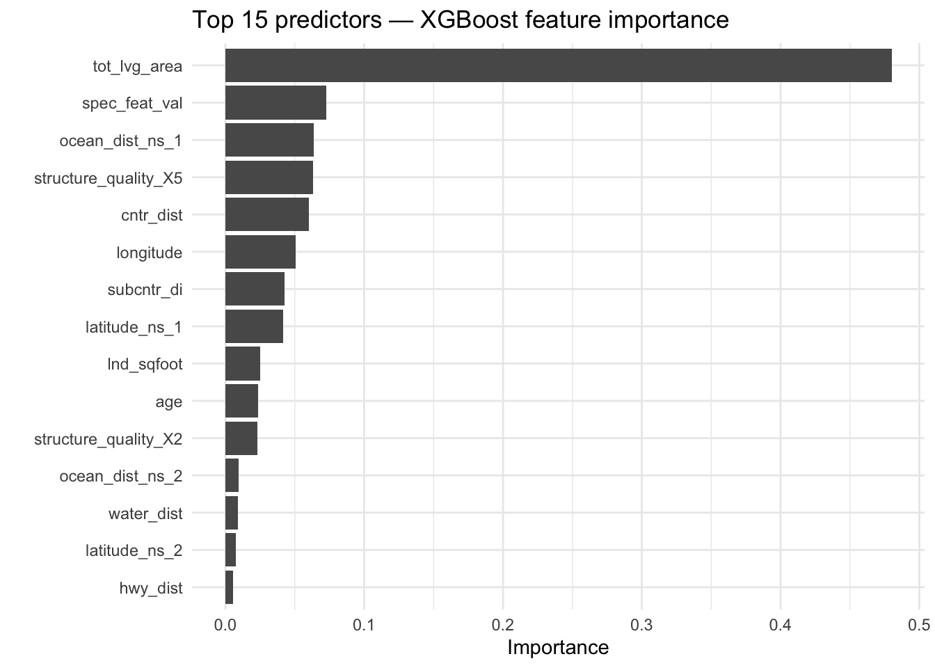
Ocean distance is the dominant predictor by a wide margin, consistent with Miami’s geography where waterfront proximity commands a significant price premium. Latitude and longitude rank highly, capturing neighborhood-level price variation that distance variables alone cannot fully explain. Structural quality and living area are the strongest property-level predictors, confirming that buyers weigh both location and physical characteristics heavily. Highway distance and property age contribute more modest but meaningful signal. The prominence of the EDA-engineered features, including the log-transformed highway distance and natural spline terms for latitude and ocean distance, in the top predictors validates the feature engineering approach taken in this project.